Data Sources
This is the documentation for data sources functions.
Create Synthetic Data
- sam.data_sources.synthetic_date_range(start='2016-01-01', end='2017-01-01', freq='h', max_delay=0, random_stop_freq=0, random_stop_max_length=1, seed=None)
Create a synthetic, somewhat realistic-looking array of datetimes.
Given a start time, end time, frequency, and some variables governing noise, creates an array of datetimes that is somewhat random.
The algorithm:
Generate a regular pandas date_range with start, end, and frequency
Delay each time by a uniformly chosen random number between 0 and max_delay, in seconds.
Pick a proportion random_stop_freq of times randomly. Each of these times x_i are deemed ‘stoppages’, and for each, a number between 1 and random_stop_max_length is uniformly chosen, say k_i. Then, the ‘stoppage’, the k_i next points after x_i are deleted, causing a hole in the times.
Only the times strictly smaller than end are kept. This means end is an exclusive bound.
- Parameters:
- start: str or datetime-like, optional (default=’2016-01-01’)
Left bound for generating dates.
- end: str or datetime-like, optional (default=’2017-01-01’)
Right bound for generating dates. Exclusive bound.
- freq: str or DateOffset, optional (default=’h’) (hourly)
Frequency strings can have multiples, e.g. ‘5H’. See `here for a list of frequency aliases. <https://pandas.pydata.org/pandas-docs/stable/timeseries.html#timeseries-offset-aliases`_
- max_delay: numeric, optional (default=0)
Each time is delayed by a random number of seconds, chosen between 0 and max_delay
- random_stop_freq: numeric, optional (default=0)
Number between 0 and 1. This proportion of all times are deemed as starting points of ‘stoppages’. A stoppage means that a number of points are removed from the result.
- random_stop_max_length: numeric, optional (default=1)
Each stoppage will have a randomly generated length, between 1 and random_stop_max_length. A stoppage of length k means that the first k points after the start of the stoppage are deleted.
- seed: int or 1-d array_like, optional (default=None)
seed for random noise generation. Passed through to numpy.random.seed. By default, no call to numpy.random.seed is made.
- Returns:
- rng: DatetimeIndex
A pandas datetimeindex of noisy times
Examples
>>> # Generate times with point approximately every 6 hours
>>> from sam.data_sources.synthetic_data import synthetic_date_range
>>> synthetic_date_range('2016-01-01', '2016-01-02', '6h', 600, 0, 1, seed=0)
DatetimeIndex(['2016-01-01 00:05:29.288102356',
               '2016-01-01 06:12:38.401722180',
               '2016-01-01 12:18:40.059747823',
               '2016-01-01 18:24:06.989657621'],
              dtype='datetime64[ns]', freq=None)
>>> # Generate times with very likely stops of length 1
>>> synthetic_date_range('2016-01-01', '2016-01-02', 'h', 0, 0.5, 1, seed=0)
DatetimeIndex(['2016-01-01 00:00:00', '2016-01-01 01:00:00',
               '2016-01-01 02:00:00', '2016-01-01 03:00:00',
               '2016-01-01 04:00:00', '2016-01-01 05:00:00',
               '2016-01-01 09:00:00', '2016-01-01 10:00:00',
               '2016-01-01 11:00:00', '2016-01-01 13:00:00',
               '2016-01-01 16:00:00', '2016-01-01 21:00:00'],
              dtype='datetime64[ns]', freq=None)
- sam.data_sources.synthetic_timeseries(dates, monthly=0, daily=0, hourly=0, monthnoise=(None, 0), daynoise=(None, 0), noise={}, minmax_values=None, cutoff_values=None, negabs=None, random_missing=None, seed=None)
Create a synthetic time series, with some temporal patterns, and some noise. There are various parameters to control the distribution of the variables. The output will never be completely realistic, it will at least resemble what real life data could look like.
The algorithm works like this:
3 cubic splines are created: one with a monthly pattern, one with a day-of-week pattern, and one with an hourly pattern. These splines are added together.
For each month and day of the week, noise is generated according to monthnoise and daynoise These two sources of noise are added together
Noise as specified by the noise parameter is generated for each point
The above three series are added together. Rescale the result according to minmax_values
Missing values are added according to cutoff_values and random_missing
The values are mutated according to negabs
The result is returned in a numpy array with the same length as the dates input. Due to the way the cubic splines are generated, there may be several dozen to a hundred data points at the beginning and end that are nan. To fix this, choose a dates array that is a couple of days longer than what you really want. Then, at the end, filter the output to only the dates in the middle.
- Parameters:
- dates: series of datetime, shape=(n_inputs,)
The index of the time series that will be created. At least length 2. Must be a pandas series, with a .dt attribute.
- monthly: numeric, optional (default=0)
The magnitude of the (random) monthly pattern. A random magnitude will be created for each month, with a cubic spline interpolating between months. The higher this value, the stronger the monthly pattern
- daily: numeric, optional (default=0)
The magnitude of the (random) daily pattern. A random magnitude will be created for each day of the week, with a cubic spline interpolating between days. The higher this value, the stronger the daily pattern
- hourly: numeric, optional (default=0)
The magnitude of the (random) hourly pattern. A random magnitude will be created for each hour, with a cubic spline interpolating between days. The higher this value, the stronger the daily pattern
- monthnoise: tuple of (str, numeric), optional (default=(None, 0))
The type and magnitude of the monthly noise. For each month, a different magnitude will be uniformly drawn between 0 and monthnoise[1]. The type of the noise is given in monthnoise[0] and is either ‘normal’, ‘poisson’, or other (no noise). This noise is added to all points,but the magnitude wil differ between the 12 different months.
- daynoise: tuple of (str, numeric), optional (default=(None, 0))
The type and magnitude of the daily noise. For each day of the week, a different magnitude will be drawn between 0 and daynoise[1]. The type of the noise is given in daynoise[0] and is either ‘normal’, ‘poisson’, or other (no noise). This noise is added to all points, but the magnitude wil differ between the 7 different days of the week.
- noise: dict, optional (default={})
The types of noise that are added to every single point. The keys of this dictionary are ‘normal’, ‘poisson’, or other (ignored) The value of the dictionary is the scale of the noise, standard deviation for normal noise, and the lambda value for poisson noise. The greater, the higher the variance of the result.
- minmax_values: tuple, optional (default=None)
The values will be linearly rescaled to always fall within these bounds. By default, no rescaling is done.
- cutoff_values: tuple, optional (default=None)
After rescaling, all the values that fall outside of these bounds will be set to nan. By default, no cutoff is done, and no values will be set to nan.
- negabs: numeric, optional (default=None)
This value is subtracted from all the output (after rescaling), and then the result will be the absolute value. This oddly-specific operation is useful in case you want a positive value that has a lot of values around 0. This is very hard to do otherwise. By subtracting and taking the absolute value, this is achieved.
- random_missing: numeric, optional (default=None)
Between 0 and 1. The fraction of values that will be set to nan. Used to emulate time series with a lot of missing values. The missing values will be completely randomly distributed with no pattern.
- seed: int or 1-d array_like, optional (default=None)
seed for random noise generation. Passed through to numpy.random.seed. By default, no call to numpy.random.seed is made.
- Returns:
- timeseries: numpy array, shape=(n_inputs,)
A numpy array containing numbers, generated according to the provided parameters.
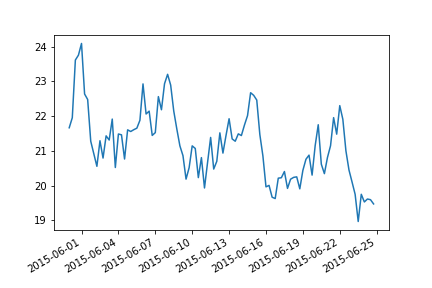
Examples
>>> # Create data that slightly resembles the temperature in a Nereda reactor:
>>> from sam.data_sources.synthetic_data import synthetic_date_range, synthetic_timeseries
>>> dates = pd.date_range('2015-01-01', '2016-01-01', freq='6H').to_series()
>>> rnd = synthetic_timeseries(
...     dates,
...     monthly=5,
...     daily=1,
...     hourly=0.0,
...     monthnoise=('normal', 0.01),
...     daynoise=('normal', 0.01),
...     noise={'normal': 0.1},
...     minmax_values=(5, 25),
...     cutoff_values=None,
...     random_missing=0.12,
...     seed = 0,
... )
>>> # visualize the result to see if it looks random or not
>>> import matplotlib.pyplot as plt
>>> fig, ax = plt.subplots()
>>> ax = ax.plot(dates[600:700], rnd[600:700])
>>> fig = fig.autofmt_xdate()
>>> plt.show()
Read Weather API’s
- sam.data_sources.read_knmi_stations()
Function to get all KNMI stations from API
- sam.data_sources.read_knmi_station_data(start_date='2021-01-01', end_date='2021-01-02', stations=None, freq='daily', variables='default', parse=True, preprocess=True)
Read KNMI data for specific station To find station numbers, use sam.data_sources.read_knmi_stations, or use sam.data_sources.read_knmi to use lat/lon and find closest station
Source: https://www.knmi.nl/kennis-en-datacentrum/achtergrond/data-ophalen-vanuit-een-script
- Parameters:
- start_datestr or datetime-like
the start time of the period from which to export weather if str, must be in the format %Y-%m-%d %H:%M:%S or %Y-%m-%d
- end_datestr or datetime-like
the end time of the period from which to export weather if str, must be in the format %Y-%m-%d %H:%M:%S or %Y-%m-%d
- stationsint, string, list or None
station number or list of station numbers, either int or string if None, data from all stations is returned
- freqstr, optional (default = ‘daily’)
frequency of export. Must be ‘hourly’ or ‘daily’
- variablesstr, None or list, optional (default=’default’)
knmi-variables to export. See all hourly variables here or all daily variables here by default, export [average temperature, sunshine duration, rainfall], which is [‘RH’, ‘SQ’, ‘T’] for hourly, and [‘RH’, ‘SQ’, ‘TG’] for daily If None, all variables will be collected
- preprocessbool, optional (default=False)
by default (False), return variables in default units (often 0.1 mm). If true, data is scaled to whole units, and default values of -1 are mapped to 0
- parsebool, optional (default=True)
if True, parse the data to a pandas dataframe Only use False for debugging purposes
- Returns
- ——-
- knmi: dataframe
Dataframe with columns as in ‘variables’, and STN, TIME columns
- sam.data_sources.read_knmi(start_date, end_date, latitude=52.11, longitude=5.18, freq='hourly', variables='default', find_nonan_station=False, preprocess=False, drop_station=True)
Export historic variables from KNMI, either hourly or daily. There are many weather stations in the Netherlands, but this function will select the station that is physically closest to the desired location, and use that station. knmi only has historic data. Usually, the most recent datapoint is about half a day prior to the current time. If the start_date and/or end_date is after the most recent available datapoint, any datapoints that are not available will not be included in the results, not even as missing data.
- Parameters:
- start_datestr or datetime-like
the start time of the period from which to export weather if str, must be in the format %Y-%m-%d %H:%M:%S or %Y-%m-%d
- end_datestr or datetime-like
the end time of the period from which to export weather if str, must be in the format %Y-%m-%d %H:%M:%S or %Y-%m-%d
- latitudefloat, optional (default=52.11)
latitude of the location from which to export weather. By default, use location of weather station De Bilt
- longitudefloat, optional (default=5.18)
longitude of the location from which to export weather. By default, use location of weather station De Bilt
- freq: str, optional (default = ‘hourly’)
frequency of export. Must be ‘hourly’ or ‘daily’
- variables: str, None or list, optional (default=’default’)
knmi-variables to export. See all hourly variables here or all daily variables here by default, export [average temperature, sunshine duration, rainfall], which is [‘RH’, ‘SQ’, ‘T’] for hourly, and [‘RH’, ‘SQ’, ‘TG’] for daily If None, all variables will be collected
- find_nonan_stationbool, optional (defaut=False)
by default (False), return the closest stations even if it includes nans. If True, return the closest station that does not include nans instead
- preprocessbool, optional (default=False)
by default (False), return variables in default units (often 0.1 mm). If true, data is scaled to whole units, and default values of -1 are mapped to 0
- drop_stationbool, optional (default=True)
by default (True), drop ‘STN’ column from result. If False, the returned dataframe will contain a column STN with station number This station number will be the same for all rows since this function returns only data for the closest station. To get data of multiple stations, try read_knmi_station_data
- Returns:
- knmi: dataframe
Dataframe with columns as in ‘variables’, and TIME column
Examples
>>> read_knmi('2018-01-01 00:00:00', '2018-01-01 06:00:00', 52.09, 5.09, 'hourly', ['SQ', 'T'])
    SQ     T                TIME
0  0.0  87.0 2018-01-01 00:00:00
1  0.0  85.0 2018-01-01 01:00:00
2  0.0  71.0 2018-01-01 02:00:00
3  0.0  78.0 2018-01-01 03:00:00
4  0.0  80.0 2018-01-01 04:00:00
5  0.0  75.0 2018-01-01 05:00:00
6  0.0  69.0 2018-01-01 06:00:00
- sam.data_sources.read_openweathermap(latitude=52.11, longitude=5.18)
Use openweathermap API to obtain a weather forecast. This forecast has a frequency of 3 hours, with a total of 39 observations, meaning the forecast is up to 5 days in the future. The resulting timestamp always uses UTC.
- Parameters:
- latitude: float, optional (default=52.11)
latitude of the location from which to export weather. By default, use location of weather station De Bilt
- longitude: float, optional (default=5.18)
longitude of the location from which to export weather. By default, use location of weather station De Bilt
- Returns:
- forecast: dataframe with TIME column, containing the time of that specific forecast,
with timezone UTC. And the following columns:
cloud_coverage, in %
humidity, in %
pressure: generally same as pressure_sealevel, in hPa
pressure_groundlevel, in hPa
pressure_sealevel, in hPa
temp, in celcius
temp_max, in celcius
temp_min, in celcius
rain_3h: volume of the last 3h, in mm
wind_deg: wind direction in degrees (meteorological)
wind_speed, in meter/sec
Examples
>>> read_openweathermap(52.11, 5.18)
    cloud_coverage  pressure_groundlevel    humidity        pressure        pressure_sealevel       temp    temp_max                    temp_min    rain_3h wind_deg        wind_speed      TIME
0   92      991.91  95      992.77  992.77  8.82    8.82    7.20    1.005   225.510 11.82   2019-03-07 15:00:00
1   92      991.57  91      992.55  992.55  8.01    8.01    6.79    0.280   223.501 13.01   2019-03-07 18:00:00
...
39  80      1009.42 73      1010.39 1010.39 8.41    8.41    8.41    0.090   204.502 10.28   2019-03-12 12:00:00
- sam.data_sources.read_regenradar(start_date: str, end_date: str, latitude: float = 52.0237687, longitude: float = 5.5920412, freq: float = '5min', batch_size: str = '7D', crs: str = 'EPSG:4326', **kwargs) DataFrame
Export historic precipitation from Nationale Regenradar.
By default, this function collects the best-known information for a single point, given by latitude and longitude in coordinate system EPSG:4326 (WGS84). This can be configured using **kwargs, but this requires some knowledge of the underlying API.
The parameters agg=average, rasters=730d6675, srs=EPSG:4326m are given to the API, as well as start, end, window given by start_date, end_date, freq. Lastly geom, which is POINT+(latitude+longitude). Alternatively, a different geometry can be passed via the geom argument in **kwargs. A different coordinate system can be passed via the srs argument in **kwargs. This is a WKT string. For example: geom=’POINT+(191601+500127)’, srs=’epsg:28992’. Exact information about the API specification and possible arguments is unfortunately unknown.
- Parameters:
- start_date: str or datetime-like
the start time of the period from which to export weather if str, must be in the format %Y-%m-%d or %Y-%m-%d %H:%M:%S
- end_date: str or datetime-like
the end time of the period from which to export weather if str, must be in the format %Y-%m-%d or %Y-%m-%d %H:%M:%S
- latitude: float, optional (default=52.11)
latitude of the location from which to export weather. By default, use location of weather station De Bilt
- longitude: float, optional (default=5.18)
longitude of the location from which to export weather. By default, use location of weather station De Bilt
- freq: str or DateOffset, default ‘5min’
frequency of export. Minimum, and default frequency is every 5 minutes. To learn more about the frequency strings, see this link.
- batch_size: str, default ‘7D’
batch size for collecting data from the API to avoid time-out. Default is 7 days.
- crs: str, default ‘EPSG:4326’
coordinate system for provided longitude (x) and latitude (y) values (or geometry by kwargs). Default is WGS84.
- kwargs: dict
additional parameters passed in the url. Must be convertable to string. Any entries with a value of None will be ignored and not passed in the url.
- Returns:
- result: dataframe
Dataframe with column PRECIPITATION and column TIME. PRECIPITATION is the precipitation in the last 5 minutes, in mm.
Examples
>>> from sam.data_sources import read_regenradar
>>> read_regenradar('2018-01-01', '2018-01-01 00:20:00')
    TIME    PRECIPITATION
0   2018-05-01 00:00:00     0.05
1   2018-05-01 00:05:00     0.09
2   2018-05-01 00:10:00     0.09
3   2018-05-01 00:15:00     0.07
4   2018-05-01 00:20:00     0.04
>>> # Example of using alternative **kwargs
>>> # For more info about these parameters, ask regenradar experts at RHDHV
>>> read_regenradar(
...     '2018-01-01',
...     '2018-01-01 00:20:00',
...     boundary_type='MUNICIPALITY',
...     geom_id=95071,
...     geom=None,
... )
    TIME    PRECIPITATION
0   2018-05-01 00:00:00     0.00
1   2018-05-01 00:05:00     0.00
2   2018-05-01 00:10:00     0.00
3   2018-05-01 00:15:00     0.00
4   2018-05-01 00:20:00     0.00
Mongo wrapper
- class sam.data_sources.MongoWrapper(db, collection, location='localhost', port=27017, **kwargs)
Bases:
objectProvides a simple wrapper to the MongoDB layers
This class provides a wrapper for basic functionality in MongoDB. We aim to use MongoDB as storage layer between analyses and e.g. dashboarding.
- Parameters:
- db: string
Name of the database
- collection: string
the name of the collection to fetch
- location: string, optional (default=”localhost”)
Location of the database
- port: integer, optional (default=27017)
Port that the database is reachable on
- **kwargs: arbitrary keyword arguments
Passed through to pymongo.MongoClient
Methods
add(content)Get as specific collection from the database
empty()Empty the collection
get([query, as_df])Get as specific collection from the database
Examples
>>> from sam.data_sources import MongoWrapper
>>> mon = MongoWrapper('test_magweg','test_magookweg')
>>> mon.empty().add([{'test': 7}]).get()
>>> test
- add(content)
Get as specific collection from the database
- Parameters:
- content: list of dictionaries, or pandas dataframe
list of items to add to the collection
- Returns:
- resultself
- empty()
Empty the collection
- Returns:
- result: self
- get(query={}, as_df=True)
Get as specific collection from the database
- Parameters:
- query: dictionary-like, optional (default={})
dictionary of parameters to use in the query. e.g. { “address”: “Park Lane 38” }
- as_df: boolean, optional (default=True)
return the query results as a Pandas Dataframe
- Returns:
- resultpandas dataframe, or list of dictionaries
the results of the query